This tutorial can be downloaded link.
Intro Tutorial 8: Using the Finite-Field (FF) Approach to Perform GW and BSE Calculations
This tutorial shows how to couple the WEST and Qbox codes in the so-called client server mode to carry out GW and BSE calculations, within or beyond the random phase approximation (RPA), using finite-field (FF) approaches as reported in Ma et al., J. Chem. Theory Comput. 15, 154 (2019) and Nguyen et al., Phys. Rev. Lett. 122, 237402 (2019).
Step 1: Mean-field starting point
Step 1.1: Mean-field calculation using Quantum ESPRESSO
We first perform the mean-field electronic structure calculation within DFT using the Quantum ESPRESSO code.
Download the following files to your working directory:
[1]:
%%bash
wget -N -q http://www.quantum-simulation.org/potentials/sg15_oncv/upf/C_ONCV_PBE-1.2.upf
wget -N -q https://west-code.org/doc/training/C60/pw.in
wget -N -q https://west-code.org/doc/training/C60/nscf.in
We can inspect the pw.in file, the input for the pw.x code:
[2]:
%%bash
cat pw.in
&control
pseudo_dir = './'
calculation = 'scf'
wf_collect = .TRUE.
/
&system
ibrav = 0
ntyp = 1
nat = 60
ecutwfc = 20
/
&electrons
diago_full_acc = .TRUE.
/
ATOMIC_SPECIES
C 14 C_ONCV_PBE-1.2.upf
ATOMIC_POSITIONS bohr
C  6.560216999227  1.317708999068  0.000000000000
C  5.716322000011  2.686502999941 -2.213027000418
C  6.560216999227 -1.317708999068  0.000000000000
C  4.900061000384  1.363055000501 -4.347289999376
C  2.686503999607  2.213028000083 -5.716321000346
C  4.347291000932  4.900060000718 -1.363055000501
C  2.213028000083  5.716322000011 -2.686502000276
C  1.363056000166  4.347291000932 -4.900058999163
C  4.900058999163 -1.363055000501  4.347289999376
C  4.900058999163  1.363055000501  4.347289999376
C  5.716321000346 -2.686502999941  2.213027000418
C  5.716321000346  2.686502999941  2.213027000418
C  4.347291000932  4.900060000718  1.363055000501
C  2.686501000610  2.213028000083  5.716321000346
C  1.363054000835  4.347291000932  4.900058999163
C  2.213027000418  5.716322000011  2.686502000276
C  2.213027000418 -5.716322000011  2.686502000276
C  1.363054000835 -4.347291000932  4.900058999163
C  4.347291000932 -4.900060000718  1.363055000501
C  2.686501000610 -2.213028000083  5.716321000346
C  1.317706999737  0.000000000000  6.560215999562
C -1.363056000166 -4.347291000932  4.900058999163
C -2.686503999607 -2.213028000083  5.716321000346
C -1.317711000289  0.000000000000  6.560215999562
C  2.213028000083 -5.716322000011 -2.686502000276
C  0.000000000000 -6.560218000782 -1.317708999068
C  4.347291000932 -4.900060000718 -1.363055000501
C  0.000000000000 -6.560218000782  1.317708999068
C -2.213028000083 -5.716322000011  2.686502000276
C -2.213027000418 -5.716322000011 -2.686502000276
C -4.347291000932 -4.900060000718 -1.363055000501
C -4.347291000932 -4.900060000718  1.363055000501
C  4.900061000384 -1.363055000501 -4.347289999376
C  2.686503999607 -2.213028000083 -5.716321000346
C  5.716322000011 -2.686502999941 -2.213027000418
C  1.363056000166 -4.347291000932 -4.900058999163
C -1.363054000835 -4.347291000932 -4.900058999163
C  1.317711000289  0.000000000000 -6.560215999562
C -1.317706999737  0.000000000000 -6.560215999562
C -2.686501000610 -2.213028000083 -5.716321000346
C -6.560216999227 -1.317708999068  0.000000000000
C -5.716321000346 -2.686502999941 -2.213027000418
C -4.900058999163 -1.363055000501 -4.347289999376
C -6.560216999227  1.317708999068  0.000000000000
C -4.900061000384  1.363055000501  4.347289999376
C -4.900061000384 -1.363055000501  4.347289999376
C -5.716322000011 -2.686502999941  2.213027000418
C -5.716322000011  2.686502999941  2.213027000418
C -2.213028000083  5.716322000011  2.686502000276
C -1.363056000166  4.347291000932  4.900058999163
C -2.686503999607  2.213028000083  5.716321000346
C -4.347291000932  4.900060000718  1.363055000501
C -2.213027000418  5.716322000011 -2.686502000276
C  0.000000000000  6.560218000782 -1.317708999068
C  0.000000000000  6.560218000782  1.317708999068
C -4.347291000932  4.900060000718 -1.363055000501
C -4.900058999163  1.363055000501 -4.347289999376
C -2.686501000610  2.213028000083 -5.716321000346
C -1.363054000835  4.347291000932 -4.900058999163
C -5.716321000346  2.686502999941 -2.213027000418
K_POINTS gamma
CELL_PARAMETERS bohr
30.0 0.0 0.0
0.0 30.0 0.0
0.0 0.0 30.0
We run pw.x on 32 cores.
[ ]:
%%bash
mpirun -n 32 pw.x -i pw.in > pw.out
To include a few unoccupied bands (in this case 800 bands in total) we run a non-self-consistent calculation. The content of nscf.in is almost identical to that of pw.in, except that in nscf.in we request a non-self-consistent calculation with empty bands.
We run pw.x again on 32 cores.
[ ]:
%%bash
mpirun -n 32 pw.x -i nscf.in > nscf.out
Step 1.2: Mean-field calculation using Qbox
Next we repeat the mean-field electronic structure calculation using the Qbox code.
Download the following files to your working directory:
[3]:
%%bash
wget -N -q https://west-code.org/doc/training/C60/qb.in
wget -N -q http://www.quantum-simulation.org/potentials/sg15_oncv/xml/C_ONCV_PBE-1.2.xml
We can inspect the qb.in file, the input for the qb code:
[4]:
%%bash
cat qb.in
set cell 30.0 0.0 0.0  0.0 30.0 0.0  0.0 0.0 30.0
species carbon C_ONCV_PBE-1.2.xml
atom C1 carbon  6.560216999227  1.317708999068  0.000000000000
atom C2 carbon  5.716322000011  2.686502999941 -2.213027000418
atom C3 carbon  6.560216999227 -1.317708999068  0.000000000000
atom C4 carbon  4.900061000384  1.363055000501 -4.347289999376
atom C5 carbon  2.686503999607  2.213028000083 -5.716321000346
atom C6 carbon  4.347291000932  4.900060000718 -1.363055000501
atom C7 carbon  2.213028000083  5.716322000011 -2.686502000276
atom C8 carbon  1.363056000166  4.347291000932 -4.900058999163
atom C9 carbon  4.900058999163 -1.363055000501  4.347289999376
atom C10 carbon  4.900058999163  1.363055000501  4.347289999376
atom C11 carbon  5.716321000346 -2.686502999941  2.213027000418
atom C12 carbon  5.716321000346  2.686502999941  2.213027000418
atom C13 carbon  4.347291000932  4.900060000718  1.363055000501
atom C14 carbon  2.686501000610  2.213028000083  5.716321000346
atom C15 carbon  1.363054000835  4.347291000932  4.900058999163
atom C16 carbon  2.213027000418  5.716322000011  2.686502000276
atom C17 carbon  2.213027000418 -5.716322000011  2.686502000276
atom C18 carbon  1.363054000835 -4.347291000932  4.900058999163
atom C19 carbon  4.347291000932 -4.900060000718  1.363055000501
atom C20 carbon  2.686501000610 -2.213028000083  5.716321000346
atom C21 carbon  1.317706999737  0.000000000000  6.560215999562
atom C22 carbon -1.363056000166 -4.347291000932  4.900058999163
atom C23 carbon -2.686503999607 -2.213028000083  5.716321000346
atom C24 carbon -1.317711000289  0.000000000000  6.560215999562
atom C25 carbon  2.213028000083 -5.716322000011 -2.686502000276
atom C26 carbon  0.000000000000 -6.560218000782 -1.317708999068
atom C27 carbon  4.347291000932 -4.900060000718 -1.363055000501
atom C28 carbon  0.000000000000 -6.560218000782  1.317708999068
atom C29 carbon -2.213028000083 -5.716322000011  2.686502000276
atom C30 carbon -2.213027000418 -5.716322000011 -2.686502000276
atom C31 carbon -4.347291000932 -4.900060000718 -1.363055000501
atom C32 carbon -4.347291000932 -4.900060000718  1.363055000501
atom C33 carbon  4.900061000384 -1.363055000501 -4.347289999376
atom C34 carbon  2.686503999607 -2.213028000083 -5.716321000346
atom C35 carbon  5.716322000011 -2.686502999941 -2.213027000418
atom C36 carbon  1.363056000166 -4.347291000932 -4.900058999163
atom C37 carbon -1.363054000835 -4.347291000932 -4.900058999163
atom C38 carbon  1.317711000289  0.000000000000 -6.560215999562
atom C39 carbon -1.317706999737  0.000000000000 -6.560215999562
atom C40 carbon -2.686501000610 -2.213028000083 -5.716321000346
atom C41 carbon -6.560216999227 -1.317708999068  0.000000000000
atom C42 carbon -5.716321000346 -2.686502999941 -2.213027000418
atom C43 carbon -4.900058999163 -1.363055000501 -4.347289999376
atom C44 carbon -6.560216999227  1.317708999068  0.000000000000
atom C45 carbon -4.900061000384  1.363055000501  4.347289999376
atom C46 carbon -4.900061000384 -1.363055000501  4.347289999376
atom C47 carbon -5.716322000011 -2.686502999941  2.213027000418
atom C48 carbon -5.716322000011  2.686502999941  2.213027000418
atom C49 carbon -2.213028000083  5.716322000011  2.686502000276
atom C50 carbon -1.363056000166  4.347291000932  4.900058999163
atom C51 carbon -2.686503999607  2.213028000083  5.716321000346
atom C52 carbon -4.347291000932  4.900060000718  1.363055000501
atom C53 carbon -2.213027000418  5.716322000011 -2.686502000276
atom C54 carbon  0.000000000000  6.560218000782 -1.317708999068
atom C55 carbon  0.000000000000  6.560218000782  1.317708999068
atom C56 carbon -4.347291000932  4.900060000718 -1.363055000501
atom C57 carbon -4.900058999163  1.363055000501 -4.347289999376
atom C58 carbon -2.686501000610  2.213028000083 -5.716321000346
atom C59 carbon -1.363054000835  4.347291000932 -4.900058999163
atom C60 carbon -5.716321000346  2.686502999941 -2.213027000418

set xc PBE
set ecut 20
set wf_dyn JD

set scf_tol 1e-08

randomize_wf 0.01
set wf_dyn PSDA
run -atomic_density 0 100 10

set wf_diag T
run 0
save qb.gs.xml
We use the same atomic positions, exchange-correlation functional, cutoff energy, and pseudopotential for qb as used for pw.x in the previous step. Check out the Qbox documentation for more information about how to operate the code.
We run qb on 32 cores.
[ ]:
%%bash
mpirun -n 32 qb < qb.in > qb.out
The information of the ground state calculation, including the Kohn-Sham wavefunctions, is stored in the file qb.gs.xml. To accelerate the BSE calculation, we localize the ground state wavefunctions using the recursive subspace bisection technique implemented in Qbox. Download the input file to your working directory:
[5]:
%%bash
wget -N -q https://west-code.org/doc/training/C60/qb2.in
We can inspect the qb2.in file:
[6]:
%%bash
cat qb2.in
load qb.gs.xml

bisection 5 5 5 0.0316
save qb.bis.0.0316.xml

set xc HF
set btHF 0.0316
set blHF 5 5 5

set wf_dyn LOCKED

run 0
We run qb again on 32 cores.
[ ]:
%%bash
mpirun -n 32 qb < qb2.in > qb2.out
qb will localize the wavefunctions stored in qb.gs.xml, then write the localized wavefunctions to the file qb.bis.0.0316.xml. We use the WESTpy Python package to parse the Qbox output files.
[ ]:
from westpy.bse import *

qb = Qbox2BSE("qb2.out")
qb.write_localization()
qb.write_wavefunction()
This generates two files, namely bis_info.1 containing bisection localization information and qb_wfc.1 containing localized wavefunctions in the HDF5 format. The extension, .1, denotes the spin channel. Both files will be used in the BSE calculation.
Step 2: GW calculation
Step 2.1: Calculation of dielectric screening using WEST-Qbox coupling
We compute the static dielectric screening using the wstat.x executable. Download the following file to your working directory:
[7]:
%%bash
wget -N -q https://west-code.org/doc/training/C60/wstat.in
Let us inspect the wstat.in file:
[8]:
%%bash
cat wstat.in
input_west:
  outdir: ./

wstat_control:
  wstat_calculation: SE
  n_pdep_eigen: 720

server_control:
  document: {"response": {"amplitude": 0.001, "nitscf": 50, "nite": 5, "approximation": RPA}, "script": ["load ./qb.gs.xml \n set xc PBE \n"]}
The wstat_calculation: SE keyword means Start from scratch and External, i.e., the calculation is outsourced to Qbox. The document keyword contains the specifics of running WEST and Qbox in the client-server mode. In this mode, we run wstat.x together with multiple instances of qb. To evaluate density response functions, the client, wstat.x, dispatches finite field calculations to the server, qb. Each instance of qb computes the density response to the
finite electric field. The same calculation can be done without resorting to the RPA, simply by taking out the "approximation": RPA part from document.

An example script to run such a calculation looks as follows:
[ ]:
%%bash
nimages=8

# Submit nimages instances of Qbox (each instance runs on 32 cores)

for (( i=0; i<$nimages; i++ ))
do
    qb_in=`printf "qb.%d.in" $i`
    qb_out=`printf "qb.%d.out" $i`
    mpirun -n 32 ./qb -server $qb_in $qb_out &
    sleep 1
done

# Submit 1 instance of WEST (it runs on 32 cores)
mpirun -n 32 ./wstat.x -ni $nimages -i wstat.in > wstat.out &
wait
The user must request computational resources for wstat.x and all instances of qb. In this example, we run wstat.x with eight instances of qb, requesting \(32 \times (1+8) = 288\) cores.
Step 2.2: Calculation of quasiparticle corrections using WEST
Now we run the wfreq.x executable to compute the quasiparticle corrections. Download the following file to your working directory:
[9]:
%%bash
wget -N -q https://west-code.org/doc/training/C60/wfreq.in
Let us inspect the wfreq.in file:
[10]:
%%bash
cat wfreq.in
input_west:
  outdir: ./

wstat_control:
  wstat_calculation: SE
  n_pdep_eigen: 720

server_control:
  document: {"response": {"amplitude": 0.001, "nitscf": 50, "nite": 5, "approximation": RPA}, "script": ["load ./qb.gs.xml \n set xc PBE \n"]}

wfreq_control:
  wfreq_calculation: XWGQ
  n_pdep_eigen_to_use: 720
  qp_bandrange: [101,140]
In the wfreq_control section, there are no input keywords specific to the FF method.
We run wfreq.x on 512 cores:
[ ]:
%%bash
mpirun -n 512 ./wfreq.x -ni 16 -i wfreq.in > wfreq.out
The reader is encouraged to repeat Step 2 using the PDEP method and compare the quasiparticle energies.
Step 3: BSE calculation
Step 3.1: BSE initialization using WEST-Qbox coupling
We perform an initialization step to compute the screened exchange integrals using the wbse_init.x executable. Download the following file to your working directory:
[11]:
%%bash
wget -N -q https://west-code.org/doc/training/C60/wbse_init.in
Let us inspect the wbse_init.in file:
[12]:
%%bash
cat wbse_init.in
input_west:
  outdir: ./

wbse_init_control:
  wbse_init_calculation: S
  bse_method: FF_Qbox
  localization: B

server_control:
  document: {"response": {"amplitude": 0, "nitscf": 20, "nite": 0}, "script": ["load ./qb.gs.xml \n set xc PBE \n set wf_dyn PSDA \n set blHF 2 2 2 \n set btHF 0.00 \n"]}
The bse_method: FF_Qbox keyword selects the FF method to solve the BSE. The localization: B keyword instructs the code to use wavefunctions localized by the recursive subspace bisection method implemented in Qbox. If two localized wavefunctions do not overlap with each other, the evaluation of the corresponding screened exchange integral is skipped, thus reducing the computational cost. Localized wavefunctions and bisection information are read from files bis_info.1 and qb_wfc.1
obtained in Step 1.2.
The document keyword is used to run WEST and Qbox in the client-server mode. But as opposed to Step 2.1, "approximation": RPA is not specified, allowing for a calculation beyond the RPA. An example script to run this calculation looks as follows:
[ ]:
%%bash
nimages=8

# Submit nimages instances of Qbox (each instance runs on 32 cores)

for (( i=0; i<$nimages; i++ ))
do
    qb_in=`printf "qb.%d.in" $i`
    qb_out=`printf "qb.%d.out" $i`
    mpirun -n 32 ./qb -server $qb_in $qb_out &
    sleep 1
done

# Submit 1 instance of WEST (it runs on 32 cores)
mpirun -n 32 ./wbse_init.x -ni $nimages -i wbse_init.in > wbse_init.out &
wait
Again, the user must request computational resources for wbse_init.x and all instances of qb.
Step 3.2: BSE absorption spectrum using WEST
Now we run the wbse.x executable to compute the absorption spectrum of C60. Download the following file to your working directory:
[13]:
%%bash
wget -N -q https://west-code.org/doc/training/C60/wbse.in
Let us inspect the wbse.in file:
[14]:
%%bash
cat wbse.in
input_west:
  outdir: ./

wbse_init_control:
  wbse_init_calculation: S
  bse_method: FF_Qbox
  localization: B

server_control:
  document: {"response": {"amplitude": 0, "nitscf": 20, "nite": 0}, "script": ["load ./qb.gs.xml \n set xc PBE \n set wf_dyn PSDA \n set blHF 2 2 2 \n set btHF 0.00 \n"]}

wbse_control:
  wbse_calculation: L
  qp_correction: west.wfreq.save/wfreq.json
  wbse_ipol: XYZ
  n_lanczos: 1300
In the wbse_control section, there are no input keywords specific to the FF method.
We run wbse.x on 512 cores:
[ ]:
%%bash
mpirun -n 512 ./wbse.x -ni 16 -i wbse.in > wbse.out
The output can be found in the file west.wbse.save/wbse.json. If the reader does NOT have the computational resources to run the calculations, the output file can be directly downloaded as:
[15]:
%%bash
mkdir -p west.wbse.save
wget -N -q https://west-code.org/doc/training/C60/wbse.json -O west.wbse.save/wbse.json
We use WESTpy to parse this file and plot the absorption coefficient as a function of the photon frequency.
[16]:
from westpy.bse import *

wbse = BSEResult("west.wbse.save/wbse.json")
wbse.plotSpectrum(ipol="XYZ",energyRange=[0.0,10.0,0.01],sigma=0.1,n_extra=98700)
 _    _ _____ _____ _____
| |  | |  ___/  ___|_   _|
| |  | | |__ \ `--.  | |_ __  _   _
| |/\| |  __| `--. \ | | '_ \| | | |
\  /\  / |___/\__/ / | | |_) | |_| |
 \/  \/\____/\____/  \_/ .__/ \__, |
                       | |     __/ |
                       |_|    |___/

WEST version     :  5.2.0
Today            :  2023-02-23 14:55:04.600349
output written in :  chi_XYZ.png
waiting for user to close image preview...
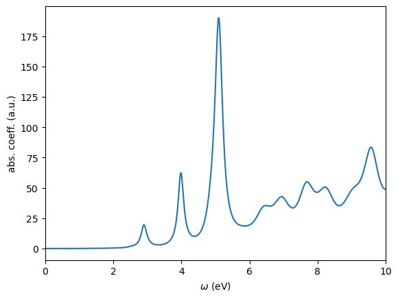
It can be verified that the FF method used in this tutorial and the PDEP method used in Tutorial 7 yield virtually identical absorption spectra.