This tutorial can be downloaded link.

Intro Tutorial 6: Identification of Localized States

In this tutorial, we show how to identify Kohn-Sham states that are localized in real space. We will identify defect orbitals of the NV\(^-\) center in diamond based on the localization factor, defined as

\[L_n = \int_{V \in \Omega} d^3\mathbf{r} \left| \psi^{\text{KS}}_n(\mathbf{r}) \right|^2\]

It describes the localization of the n-th KS wavefunction in a given volume \(V\) within the supercell volume \(\Omega\). The volume \(V\) can be a box or a sphere.

More details can be found in N. Sheng, C. Vorwerk, M. Govoni, and G. Galli, J. Chem. Theory Comput. 18, 3512 (2022).

Step 1: Mean-field starting point

We perform the mean-field electronic structure calculation within density-functional theory (DFT) using the Quantum ESPRESSO code.

Download the following files in your working directory:

%%bash
wget -N -q https://west-code.org/doc/training/nv_diamond_63/pw.in
wget -N -q http://www.quantum-simulation.org/potentials/sg15_oncv/upf/C_ONCV_PBE-1.2.upf
wget -N -q http://www.quantum-simulation.org/potentials/sg15_oncv/upf/N_ONCV_PBE-1.2.upf

We inspect the pw.in file, the input for the pw.x code:

%%bash
cat pw.in

&CONTROL
calculation = 'scf'
pseudo_dir = './'
/
&SYSTEM
input_dft = 'PBE'
ibrav = 0
ecutwfc = 50
tot_charge = -1
nspin = 1
nbnd = 176
occupations = 'from_input'
nat = 63
ntyp = 2
/
&ELECTRONS
diago_full_acc = .true.
/
K_POINTS gamma
CELL_PARAMETERS angstrom
7.136012  0.000000  0.000000
0.000000  7.136012  0.000000
0.000000  0.000000  7.136012
ATOMIC_SPECIES
C  12.01099968  C_ONCV_PBE-1.2.upf
N  14.00699997  N_ONCV_PBE-1.2.upf
ATOMIC_POSITIONS crystal
C    0.99996000  0.99996000  0.99996000
C    0.12495000  0.12495000  0.12495000
C    0.99905000  0.25039000  0.25039000
C    0.12350000  0.37499000  0.37499000
C    0.25039000  0.99905000  0.25039000
C    0.37499000  0.12350000  0.37499000
C    0.25039000  0.25039000  0.99905000
C    0.37499000  0.37499000  0.12350000
C    0.00146000  0.00146000  0.50100000
C    0.12510000  0.12510000  0.62503000
C    0.00102000  0.24944000  0.74960000
C    0.12614000  0.37542000  0.87402000
C    0.24944000  0.00102000  0.74960000
C    0.37542000  0.12614000  0.87402000
C    0.24839000  0.24839000  0.49966000
C    0.37509000  0.37509000  0.61906000
C    0.00146000  0.50100000  0.00146000
C    0.12510000  0.62503000  0.12510000
C    0.00102000  0.74960000  0.24944000
C    0.12614000  0.87402000  0.37542000
C    0.24839000  0.49966000  0.24839000
C    0.37509000  0.61906000  0.37509000
C    0.24944000  0.74960000  0.00102000
C    0.37542000  0.87402000  0.12614000
C    0.99883000  0.50076000  0.50076000
C    0.12502000  0.62512000  0.62512000
C    0.99961000  0.74983000  0.74983000
C    0.12491000  0.87493000  0.87493000
C    0.25216000  0.50142000  0.74767000
C    0.37740000  0.62659000  0.87314000
C    0.25216000  0.74767000  0.50142000
C    0.37740000  0.87314000  0.62659000
C    0.50100000  0.00146000  0.00146000
C    0.62503000  0.12510000  0.12510000
C    0.49966000  0.24839000  0.24839000
C    0.61906000  0.37509000  0.37509000
C    0.74960000  0.00102000  0.24944000
C    0.87402000  0.12614000  0.37542000
C    0.74960000  0.24944000  0.00102000
C    0.87402000  0.37542000  0.12614000
C    0.50076000  0.99883000  0.50076000
C    0.62512000  0.12502000  0.62512000
C    0.50142000  0.25216000  0.74767000
C    0.62659000  0.37740000  0.87314000
C    0.74983000  0.99961000  0.74983000
C    0.87493000  0.12491000  0.87493000
C    0.74767000  0.25216000  0.50142000
C    0.87314000  0.37740000  0.62659000
C    0.50076000  0.50076000  0.99883000
C    0.62512000  0.62512000  0.12502000
C    0.50142000  0.74767000  0.25216000
C    0.62659000  0.87314000  0.37740000
C    0.74767000  0.50142000  0.25216000
C    0.87314000  0.62659000  0.37740000
C    0.74983000  0.74983000  0.99961000
C    0.87493000  0.87493000  0.12491000
N    0.48731000  0.48731000  0.48731000
C    0.49191000  0.76093000  0.76093000
C    0.62368000  0.87476000  0.87476000
C    0.76093000  0.49191000  0.76093000
C    0.87476000  0.62368000  0.87476000
C    0.76093000  0.76093000  0.49191000
C    0.87476000  0.87476000  0.62368000
OCCUPATIONS
2 2 2 2 2 2 2 2 2 2
2 2 2 2 2 2 2 2 2 2
2 2 2 2 2 2 2 2 2 2
2 2 2 2 2 2 2 2 2 2
2 2 2 2 2 2 2 2 2 2
2 2 2 2 2 2 2 2 2 2
2 2 2 2 2 2 2 2 2 2
2 2 2 2 2 2 2 2 2 2
2 2 2 2 2 2 2 2 2 2
2 2 2 2 2 2 2 2 2 2
2 2 2 2 2 2 2 2 2 2
2 2 2 2 2 2 2 2 2 2
2 2 2 2 2 2 1 1 0 0
0 0 0 0 0 0 0 0 0 0
0 0 0 0 0 0 0 0 0 0
0 0 0 0 0 0 0 0 0 0
0 0 0 0 0 0 0 0 0 0
0 0 0 0 0 0

We can now run pw.x on 2 cores.

%%bash
mpirun -n 2 pw.x -i pw.in > pw.out

We have carried out a spin unpolarized calculation (i.e., nspin = 1) because we want to use \(L_n\) to define an active space for quantum defect embedding theory (QDET, see Tutorial 5). The latter uses a spin-unpolarized mean-field starting point to reduce spin contamination in the generation of the effective Hamiltonian.

Step 2.1: Calculation of the localization factor using a box

Localization factors are calculated with the westpp.x executable within WEST. You can generate the input file with the following command:

import yaml

d = {}
d['westpp_control'] = {}
d['westpp_control']['westpp_calculation'] = 'L'
d['westpp_control']['westpp_range'] = [1, 176]
d['westpp_control']['westpp_box'] = [6.19, 10.19, 6.28, 10.28, 6.28, 10.28]

with open('westpp.in', 'w') as f:
    yaml.dump(d, f, sort_keys=False)

Let us inspect the input file.

%%bash
cat westpp.in

westpp_control:
  westpp_calculation: L
  westpp_range:
  - 1
  - 176
  westpp_box:
  - 6.19
  - 10.19
  - 6.28
  - 10.28
  - 6.28
  - 10.28

The keyword westpp_calculation: L triggers the calculation of the localization factor. With westpp_range, we can select for which Kohn-Sham states we compute the localization factor. In this tutorial, we use all 176 states. Finally, westpp_box specifies the parameter of a box in atomic units to use for the integration. In this case, we have chosen a cubic box around the carbon vacancy at \(\left( 8.18, 8.28, 8.28 \right)\) Bohr with an edge of 4 Bohr. The box has a volume of 64 Bohr\(^3\), which is smaller than the supercell volume of 2452.24 Bohr\(^3\).

We run westpp.x on 2 cores.

%%bash
mpirun -n 2 westpp.x -i westpp.in > westpp.out

westpp.x creates a file named west.westpp.save/westpp.json. If the reader does NOT have the computational resources to run the calculation, the WEST output file needed for the next step can be directly downloaded as:

%%bash
mkdir -p west.westpp.save
wget -N -q https://west-code.org/doc/training/nv_diamond_63/box_westpp.json -O west.westpp.save/westpp.json

We can now visualize the results:

import json
import numpy as np
import matplotlib.pyplot as plt

with open('west.westpp.save/westpp.json','r') as f:
    data = json.load(f)

y = np.array(data['output']['L']['K00001']['local_factor'],dtype='f8')
x = np.array([i+1 for i in range(y.shape[0])])

plt.plot(x,y,'o')
plt.axhline(y=0.08,linestyle='--',color='red')

plt.xlabel('KS index')
plt.ylabel('Localization factor')

plt.show()

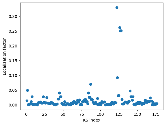
We see that a number of Kohn-Sham orbitals have a localization factor \(>0.08\).

print(x[y>=0.08])

[122 123 126 127 128]

The highest localization factor (>0.08) is found for Kohn-Sham orbitals with indices 122, 123, 126, 127, and 128.

Step 2.2: Calculation of the localization factor using a sphere

Let us modify the input file westpp.in to compute localization factors within a sphere.

import yaml

d = {}
d['westpp_control'] = {}
d['westpp_control']['westpp_calculation'] = 'L'
d['westpp_control']['westpp_range'] = [1, 176]
d['westpp_control']['westpp_format'] = 'S'
d['westpp_control']['westpp_r0'] = [8.18, 8.28, 8.28]
d['westpp_control']['westpp_rmax'] = 2.4814

with open('westpp.in', 'w') as f:
    yaml.dump(d, f, sort_keys=False)

Let us inspect the input file.

%%bash
cat westpp.in

westpp_control:
  westpp_calculation: L
  westpp_range:
  - 1
  - 176
  westpp_format: S
  westpp_r0:
  - 8.18
  - 8.28
  - 8.28
  westpp_rmax: 2.4814

The keyword westpp_format: S instructs the code to compute the localization factor within a sphere, which is centered around \(\left( 8.18, 8.28, 8.28 \right)\) Bohr as specified by westpp_r0 and has a radius of 2.4814 Bohr as specified by westpp_rmax. The sphere has a volume of ~64 Bohr\(^3\), which is roughly the same as the volume of the box used in the previous section.

We run westpp.x on 2 cores.

%%bash
mpirun -n 2 westpp.x -i westpp.in > westpp.out

westpp.x creates a file named west.westpp.save/westpp.json. If the reader does NOT have the computational resources to run the calculation, the WEST output file needed for the next step can be directly downloaded as:

%%bash
mkdir -p west.westpp.save
wget -N -q https://west-code.org/doc/training/nv_diamond_63/sphere_westpp.json -O west.westpp.save/westpp.json

We can now visualize the results:

import json
import numpy as np
import matplotlib.pyplot as plt

with open('west.westpp.save/westpp.json','r') as f:
    data = json.load(f)

y = np.array(data['output']['L']['K00001']['local_factor'],dtype='f8')
x = np.array([i+1 for i in range(y.shape[0])])

plt.plot(x,y,'o')
plt.axhline(y=0.08,linestyle='--',color='red')

plt.xlabel('KS index')
plt.ylabel('Localization factor')

plt.show()

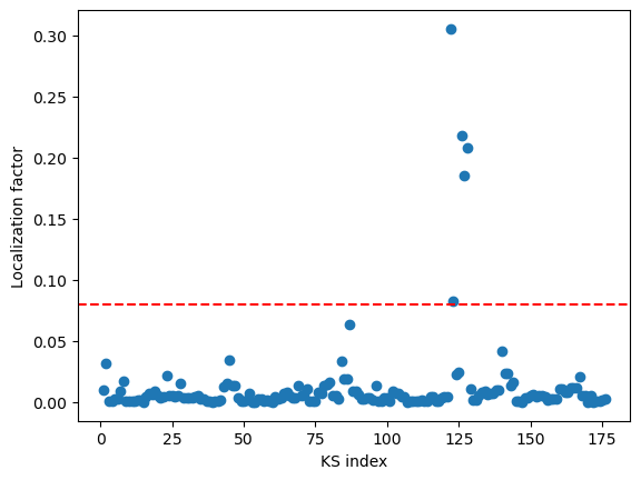
We see that a number of Kohn-Sham orbitals have a localization factor \(>0.08\).

print(x[y>=0.08])

[122 123 126 127 128]

The highest localization factor (>0.08) is found for Kohn-Sham orbitals with indices 122, 123, 126, 127, and 128, which are the same orbitals as identified by computing localization factors in a box.