MICCoM School 2017 Ex#5 : Hybrid functionals

We are going to use the SX hybrid functional in order to compute the VIP of silane.

A hybrid functional contains a mixture of semilocal (\(V_{\text{x}}\)) and exact exchange (\(V_{\text{xx}}\)):

\begin{equation} H^{\text{hyb}}= T + V_{\text{ion}} + V_{\text{Hartree}} + V_{\text{xc}} + \alpha (V_{\text{xx}}-V_{\text{x}}) \end{equation}

For the hybrid functional PBE0 \(\alpha=0.25\).

A class of dielectric dependent hybrid functionals was developed in order to make \(\alpha\) material dependent and to obtain higher accuracy. For dielectric dependent hybrid functionals \(\alpha\) is a parameter that can be determined from first principles:

• For solids (sc-hybrid functional): \(\alpha = \epsilon_\infty^{-1}\) [Phys. Rev. B 89, 195112 (2014)]

• For molecules (SX functional): \(\alpha_n = \frac{\left\langle \psi_n \right| \Sigma_{\text{SEX}} \left | \psi_n \right\rangle}{\left\langle \psi_n \right| \Sigma_{\text{EX}} \left | \psi_n \right\rangle}\) [Phys. Rev. X 6, 041002 (2016)]

where \(\Sigma_{\text{SEX}}\) is the screened exact exchange and \(\Sigma_{\text{EX}}\) is the exact exchange:

\begin{equation} \Sigma_{\text{SEX}}(\mathbf{r},\mathbf{r^\prime}) = -\sum_n^{N_{\text{states}}} \psi_n(\mathbf{r}) W(\mathbf{r},\mathbf{r^\prime}) \psi^\ast_n(\mathbf{r^\prime}) \end{equation} and \begin{equation} \Sigma_{\text{EX}}(\mathbf{r},\mathbf{r^\prime}) = -\sum_n^{N_{\text{states}}} \psi_n(\mathbf{r}) v_{Coulomb}(\mathbf{r},\mathbf{r^\prime}) \psi^\ast_n(\mathbf{r^\prime}) \end{equation}

In order to compute the SX constant we need to compute the DFT electronic structure with semilocal functionals (pw.x), compute the eigendecomposition of the dielectric screening (wstat.x), and extract the information about the screening with the WEST post-processing tool (westpp.x).

Let’s download the material.

# pseudopotentials
!wget -N -q http://www.quantum-simulation.org/potentials/sg15_oncv/upf/Si_ONCV_PBE-1.2.upf
!wget -N -q http://www.quantum-simulation.org/potentials/sg15_oncv/upf/H_ONCV_PBE-1.2.upf

# input files
!wget -N -q https://west-code.org/doc/training/silane/pw.in
!wget -N -q https://west-code.org/doc/training/silane/wstat.in
!wget -N -q https://west-code.org/doc/training/silane/westpp.in

These two steps may be familiar:

!mpirun -n 8 pw.x -i pw.in > pw.out

!mpirun -n 8 wstat.x -i wstat.in > wstat.out

5.1 The SX constant

The calculation of the SX constant is done using westpp.x.

Let’s give a quick look at the input for westpp.x (description of the input variables for westpp.x can be found here: https://west-code.org/doc/West/latest/manual.html#westpp-control).

# quick look at the input file for westpp.x
!cat westpp.in

input_west:
    qe_prefix: silane
    west_prefix: silane
    outdir: ./

wstat_control:
    wstat_calculation: S
    n_pdep_eigen: 50

westpp_control:
    westpp_calculation: S
    westpp_n_pdep_eigen_to_use: 50
    westpp_range: [1,4]

The input instructs the code to read the output of DFT and 50 eigenpotentials (previously computed using wstat.x), then extract the values of \(\left\langle \psi_n \right| \Sigma_{\text{EX}} \left | \psi_n \right\rangle\) and \(\left\langle \psi_n \right| \Sigma_{\text{SEX}} \left | \psi_n \right\rangle\) for states 1, 2, 3, and 4.

!mpirun -n 8 westpp.x -i westpp.in > westpp.out

For HOMO \(\alpha=0.758899\), let’s use it to perform a hybrid DFT calculation.

Note the addition of:

input_dft       ='PBE0'
exx_fraction    = 0.758899

in the input file for pw.x.

# write to file
with open('pw_hybrid.in', 'w') as text_file :
    text_file.write("""&control
calculation  = 'scf'
restart_mode = 'from_scratch'
pseudo_dir   = './'
outdir       = './'
prefix       = 'silane'
wf_collect   = .TRUE.
/
&system
ibrav           = 1
celldm(1)       = 20
nat             = 5
ntyp            = 2
ecutwfc         = 25.0
nbnd            = 10
assume_isolated ='mp'
input_dft       ='PBE0'
exx_fraction    = 0.758899
/
&electrons
diago_full_acc = .TRUE.
/
ATOMIC_SPECIES
Si 28.0855  Si_ONCV_PBE-1.2.upf
H  1.00794   H_ONCV_PBE-1.2.upf
ATOMIC_POSITIONS bohr
Si      10.000000   10.000000  10.000000
H       11.614581   11.614581  11.614581
H        8.385418    8.385418  11.614581
H        8.385418   11.614581   8.385418
H       11.614581    8.385418   8.385418
K_POINTS {gamma}
""")

!mpirun -n 8 pw.x -i pw_hybrid.in > pw_hybrid.out

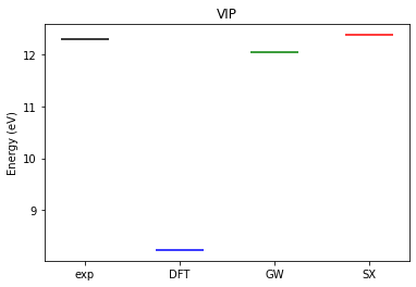
We plot the energy levels.

import numpy as np
import matplotlib.pyplot as plt

# VIP
y = {}
y['exp'] = [ 12.3 ]
y['DFT'] = [ 8.2314 ]
y['GW']  = [ 12.044023 ]
y['SX']  = [ 12.3729 ]

# colors
c = {}
c['exp'] = 'black'
c['DFT'] = 'blue'
c['GW']  = 'green'
c['SX']  = 'red'

# plot
x = list(range(1, len(y)+1))
labels = y.keys()

fig, ax = plt.subplots(1, 1)
counter = 0
for i in labels :
    for a in y[i] :
        ax.hlines(a, x[counter]-0.25, x[counter]+0.25, color=c[i])
    counter += 1

plt.xticks(x, labels)

plt.ylabel('Energy (eV)')
plt.title('VIP')

plt.show()