This tutorial can be downloaded link.
Intro Tutorial 7: Computing Absorption Spectra by Solving the Bethe-Salpeter Equation (BSE) Using Density Matrix Perturbation Theory (DMPT)
This tutorial shows how to compute the absorption spectrum of the C\(_{60}\) molecule by solving the Bethe-Salpeter Equation (BSE) using the density matrix perturbation theory (DMPT).
WEST implements two distinct methods to compute the dielectric screening for the BSE solver:
the projective dielectric eigenpotentials (PDEP) technique, which builds a low rank representation of the static dielectric matrix that enters the screened Coulomb interaction, the random phase approximation (RPA) is used;
the finite field (FF) method, which allows for efficient calculations within and beyond the RPA.
Both methods circumvent the explicit computation of empty electronic states and the storage and inversion of large matrices. In addition, the computational cost can be reduced by using a localized representation of the ground state Kohn-Sham wavefunctions.
This tutorial focuses on the PDEP-based method as described in Rocca et al., J. Chem. Phys. 133, 164109 (2010) and Rocca et al., Phys. Rev. B 85, 045116 (2012). The FF-based method is covered in Tutorial 8. Tutorial 13 shows how to compute excitation energies by solving the BSE.
Step 1: Mean-field starting point
We first perform the mean-field electronic structure calculation within DFT using the Quantum ESPRESSO code.
Download the following files to your working directory:
[1]:
%%bash
wget -N -q http://www.quantum-simulation.org/potentials/sg15_oncv/upf/C_ONCV_PBE-1.2.upf
wget -N -q https://west-code.org/doc/training/C60_pdep/pw.in
wget -N -q https://west-code.org/doc/training/C60_pdep/nscf.in
We can inspect the pw.in file, the input for the pw.x code:
[2]:
%%bash
cat pw.in
&control
pseudo_dir = './'
calculation = 'scf'
wf_collect = .TRUE.
/
&system
ibrav = 0
ntyp = 1
nat = 60
ecutwfc = 20
/
&electrons
diago_full_acc = .TRUE.
/
ATOMIC_SPECIES
C 14 C_ONCV_PBE-1.2.upf
ATOMIC_POSITIONS bohr
C  6.560216999227  1.317708999068  0.000000000000
C  5.716322000011  2.686502999941 -2.213027000418
C  6.560216999227 -1.317708999068  0.000000000000
C  4.900061000384  1.363055000501 -4.347289999376
C  2.686503999607  2.213028000083 -5.716321000346
C  4.347291000932  4.900060000718 -1.363055000501
C  2.213028000083  5.716322000011 -2.686502000276
C  1.363056000166  4.347291000932 -4.900058999163
C  4.900058999163 -1.363055000501  4.347289999376
C  4.900058999163  1.363055000501  4.347289999376
C  5.716321000346 -2.686502999941  2.213027000418
C  5.716321000346  2.686502999941  2.213027000418
C  4.347291000932  4.900060000718  1.363055000501
C  2.686501000610  2.213028000083  5.716321000346
C  1.363054000835  4.347291000932  4.900058999163
C  2.213027000418  5.716322000011  2.686502000276
C  2.213027000418 -5.716322000011  2.686502000276
C  1.363054000835 -4.347291000932  4.900058999163
C  4.347291000932 -4.900060000718  1.363055000501
C  2.686501000610 -2.213028000083  5.716321000346
C  1.317706999737  0.000000000000  6.560215999562
C -1.363056000166 -4.347291000932  4.900058999163
C -2.686503999607 -2.213028000083  5.716321000346
C -1.317711000289  0.000000000000  6.560215999562
C  2.213028000083 -5.716322000011 -2.686502000276
C  0.000000000000 -6.560218000782 -1.317708999068
C  4.347291000932 -4.900060000718 -1.363055000501
C  0.000000000000 -6.560218000782  1.317708999068
C -2.213028000083 -5.716322000011  2.686502000276
C -2.213027000418 -5.716322000011 -2.686502000276
C -4.347291000932 -4.900060000718 -1.363055000501
C -4.347291000932 -4.900060000718  1.363055000501
C  4.900061000384 -1.363055000501 -4.347289999376
C  2.686503999607 -2.213028000083 -5.716321000346
C  5.716322000011 -2.686502999941 -2.213027000418
C  1.363056000166 -4.347291000932 -4.900058999163
C -1.363054000835 -4.347291000932 -4.900058999163
C  1.317711000289  0.000000000000 -6.560215999562
C -1.317706999737  0.000000000000 -6.560215999562
C -2.686501000610 -2.213028000083 -5.716321000346
C -6.560216999227 -1.317708999068  0.000000000000
C -5.716321000346 -2.686502999941 -2.213027000418
C -4.900058999163 -1.363055000501 -4.347289999376
C -6.560216999227  1.317708999068  0.000000000000
C -4.900061000384  1.363055000501  4.347289999376
C -4.900061000384 -1.363055000501  4.347289999376
C -5.716322000011 -2.686502999941  2.213027000418
C -5.716322000011  2.686502999941  2.213027000418
C -2.213028000083  5.716322000011  2.686502000276
C -1.363056000166  4.347291000932  4.900058999163
C -2.686503999607  2.213028000083  5.716321000346
C -4.347291000932  4.900060000718  1.363055000501
C -2.213027000418  5.716322000011 -2.686502000276
C  0.000000000000  6.560218000782 -1.317708999068
C  0.000000000000  6.560218000782  1.317708999068
C -4.347291000932  4.900060000718 -1.363055000501
C -4.900058999163  1.363055000501 -4.347289999376
C -2.686501000610  2.213028000083 -5.716321000346
C -1.363054000835  4.347291000932 -4.900058999163
C -5.716321000346  2.686502999941 -2.213027000418
K_POINTS gamma
CELL_PARAMETERS bohr
30.0 0.0 0.0
0.0 30.0 0.0
0.0 0.0 30.0
We run pw.x on 32 cores.
[ ]:
%%bash
mpirun -n 32 pw.x -i pw.in > pw.out
To include a few unoccupied bands (in this case 800 bands in total) we run a non-self-consistent calculation. The content of nscf.in is almost identical to that of pw.in, except that in nscf.in we request a non-self-consistent calculation with empty bands.
We run pw.x again on 32 cores.
[ ]:
%%bash
mpirun -n 32 pw.x -i nscf.in > nscf.out
Step 2: Calculation of dielectric screening
As detailed in Tutorial 1, the static dielectric screening is computed using the projective dielectric eigendecomposition (PDEP) technique.
Download the following file to your working directory:
[3]:
%%bash
wget -N -q https://west-code.org/doc/training/C60_pdep/wstat.in
Let us inspect the wstat.in file:
[4]:
%%bash
cat wstat.in
input_west:
  outdir: ./

wstat_control:
  wstat_calculation: S
  n_pdep_eigen: 720
We run wstat.x on 512 cores:
[ ]:
%%bash
mpirun -n 512 wstat.x -ni 16 -i wstat.in > wstat.out
Step 3: BSE calculation
Step 3.1: BSE initialization
We perform an initialization step to compute the screened exchange integrals using the wbse_init.x executable.
Download the following file to your working directory:
[5]:
%%bash
wget -N -q https://west-code.org/doc/training/C60_pdep/wbse_init.in
Let us inspect the wbse_init.in file:
[6]:
%%bash
cat wbse_init.in
input_west:
  outdir: ./

wbse_init_control:
  wbse_init_calculation: S
  bse_method: PDEP
  n_pdep_eigen_to_use: 720
  localization: W
  overlap_thr: 0.001
The bse_method: PDEP keyword selects the PDEP method. A total number of n_pdep_eigen_to_use: 720 PDEPs is used to represent the static dielectric matrix. The localization: W keyword instructs the code to use Wannier functions, which are a localized representation of the Kohn-Sham wavefunctions. If the overlap between two Wannier functions is below overlap_thr: 0.001, the evaluation of the corresponding screened exchange integral is skipped, thus reducing the computational cost.
We run wbse_init.x on 512 cores:
[ ]:
%%bash
mpirun -n 512 wbse_init.x -ni 16 -i wbse_init.in > wbse_init.out
Step 3.2: BSE absorption spectrum
Now we run the wbse.x executable to compute the absorption spectrum of C\(_{60}\).
Download the following file to your working directory:
[7]:
%%bash
wget -N -q https://west-code.org/doc/training/C60_pdep/wbse.in
Let us inspect the wbse.in file:
[8]:
%%bash
cat wbse.in
input_west:
  outdir: ./

wbse_init_control:
  wbse_init_calculation: S
  bse_method: PDEP
  n_pdep_eigen_to_use: 720
  localization: W
  overlap_thr: 0.001

wbse_control:
  wbse_calculation: L
  qp_correction: west.wfreq.save/wfreq.json
  wbse_ipol: XYZ
  n_lanczos: 1300
The wbse_calculation: L keyword instructs the code to compute the absorption spectrum using the Lanczos algorithm. The wbse_ipol: XYZ keyword specifies which components of the polarizability tensor are computed, where XYZ means that three Lanczos chains are sequentially performed to compute the full polarizability tensor.
The qp_correction keyword indicates the name of the JSON file that contains the quasiparticle correction. This file is obtained from a GW calculation following the steps in Tutorial 1. An example wfreq.json file can be downloaded as:
[9]:
%%bash
mkdir -p west.wfreq.save
wget -N -q https://west-code.org/doc/training/C60_pdep/wfreq.json -O west.wfreq.save/wfreq.json
Alternatively, a scissors operator may be applied to model the quasiparticle correction, by simply replacing the qp_correction keyword with the scissor_ope keyword.
We now run wbse.x on 512 cores:
[ ]:
%%bash
mpirun -n 512 wbse.x -ni 16 -i wbse.in > wbse.out
The output can be found in the file west.wbse.save/wbse.json. If the reader does NOT have the computational resources to run the calculations, the output file can be directly downloaded as:
[10]:
%%bash
mkdir -p west.wbse.save
wget -N -q https://west-code.org/doc/training/C60_pdep/wbse.json -O west.wbse.save/wbse.json
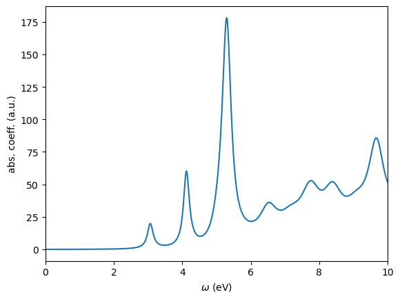
We use WESTpy to parse this file and plot the absorption coefficient as a function of the photon frequency.
[11]:
from westpy.bse import *

wbse = BSEResult("west.wbse.save/wbse.json")
wbse.plotSpectrum(ipol="XYZ",energyRange=[0.0,10.0,0.01],sigma=0.1,n_extra=98700)
 _    _ _____ _____ _____
| |  | |  ___/  ___|_   _|
| |  | | |__ \ `--.  | |_ __  _   _
| |/\| |  __| `--. \ | | '_ \| | | |
\  /\  / |___/\__/ / | | |_) | |_| |
 \/  \/\____/\____/  \_/ .__/ \__, |
                       | |     __/ |
                       |_|    |___/

WEST version     :  5.2.0
Today            :  2023-02-23 14:48:23.237369
output written in :  chi_XYZ.png
waiting for user to close image preview...