This tutorial can be downloaded link.

2.0 Analyzing the frequency dependency in GW calculations¶

We analyze the frequency dependency of the GW self-energy, by exploring two ways of solving the Quasiparticle equation:

without linearization

\begin{align} E-\varepsilon_{KS} = \langle \Sigma(E) -V_{xc} \rangle \end{align}

with linearization (first-order expansion of self-energy in the frequency domain)

\begin{align} E-\varepsilon_{KS} = \langle \Sigma(\varepsilon_{KS}) -V_{xc} \rangle + (E-\varepsilon_{KS}) \langle \frac{\partial\Sigma}{\partial E}(\varepsilon_{KS}) \rangle \end{align}

where \(\varepsilon_{KS}\) is the Kohn-Sham energy, and \(E\) is the QP energy obtained at the \(G_0W_0\) level of theory.

After completing step 1 and step 2 of the 1.0 Tutorial, we download the following file:

[1]:

%%bash
wget -N -q http://www.west-code.org/doc/training/silane/wfreq_spec.in

Let’s inspect the wfreq_spec.in file, input for wfreq.x.

[1]:

%%bash
cat wfreq_spec.in

input_west:
    qe_prefix: silane
    west_prefix: silane
    outdir: ./

wstat_control:
    wstat_calculation: S
    n_pdep_eigen: 50

wfreq_control:
    wfreq_calculation: XWGQP
    n_pdep_eigen_to_use: 50
    qp_bandrange: [4,5]
    n_refreq: 2000
    ecut_refreq: 2.0
    ecut_spectralf: [-1.5,0.5]
    n_spectralf: 2000

Run wfreq.x on 2 cores.

[ ]:

%%bash
mpirun -n 2 wfreq.x < wfreq_spec.in > wfreq_spec.out

The output file wfreq.out contains information about the calculation of the GW self-energy, and the corrected electronic structure can be found in the file <west_prefix>.wfreq.save/wfreq.json.

Below we show how to load and plot the frequency-dependent quasiparticle corrections.

[3]:

import json
import numpy as np

# Load the output data
with open('silane.wfreq.save/wfreq.json') as json_file:
    data = json.load(json_file)

# Extract converged quasiparticle (QP) corrections
k=1
kindex = f"K{k:06d}"

bandmap = data["output"]["Q"]["bandmap"]
eqp = data["output"]["Q"][kindex]

freqlist = np.array(data["output"]["P"]["freqlist"], dtype="f8")
spf = data["output"]["P"][kindex]

[10]:

# Plot
import matplotlib.pyplot as plt

for i, b in enumerate(bandmap) :

    eks, eqpLin, eqpSec = eqp['eks'][i], eqp['eqpLin'][i], eqp['eqpSec'][i]

    # Print QP corrections
    print (f"{'k':^10} | {'band':^10} | {'eks [eV]':^15} | {'eqpLin [eV]':^15} | {'eqpSec [eV]':^15}")
    print(77*"-")
    print(f"{k:^10} | {b:^10} | {eks:^15.3f} | {eqpLin:^15.3f} | {eqpSec:^15.3f}")

    sigmax, vxcl, vxcnl = eqp['sigmax'][i], eqp['vxcl'][i], eqp['vxcnl'][i]
    sigmac_eks = eqp['sigmac_eks']['re'][i]
    sigmac_eqpLin = eqp['sigmac_eqpLin']['re'][i]
    sigmac_eqpSec = eqp['sigmac_eqpSec']['re'][i]
    z = eqp['z'][i]

    bindex = f"B{b:06d}"
    sigmac = np.array(spf[bindex]['sigmac']['re'], dtype="f8")

    # Left-hand side of QP equation
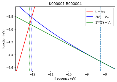
    plt.plot(freqlist,freqlist-eks,'r-',label=r"$E-\varepsilon_{KS}$")

    # Right-hand side of QP equation without linearization
    plt.plot(freqlist,sigmac+sigmax-vxcl-vxcnl,'b-',label=r"$\Sigma(E)-V_{xc}$")

    # Right-hand side of QP equation with linearization
    plt.plot(freqlist,sigmac_eks+sigmax-vxcl-vxcnl+(1-1/z)*(freqlist-eks),'g-',label=r"$\Sigma^{lin}(E)-V_{xc}$")

    plt.legend()
    plt.title(kindex+" "+bindex)
    plt.xlabel("frequency (eV)")
    plt.ylabel("function (eV)")
    xmin, xmax = min(eks, eqpLin, eqpSec), max(eks, eqpLin, eqpSec)
    ymin, ymax = min(sigmac_eks, sigmac_eqpLin, sigmac_eqpSec), max(sigmac_eks, sigmac_eqpLin, sigmac_eqpSec)
    ymin += sigmax - vxcl -vxcnl
    ymax += sigmax - vxcl -vxcnl
    plt.vlines(x=eks,ymin=ymin-0.2*(ymax-ymin),ymax=ymax+0.2*(ymax-ymin),ls="--")
    plt.vlines(x=eqpLin,ymin=ymin-0.2*(ymax-ymin),ymax=ymax+0.2*(ymax-ymin),ls=":",color="g")
    plt.vlines(x=eqpSec,ymin=ymin-0.2*(ymax-ymin),ymax=ymax+0.2*(ymax-ymin),ls=":",color="b")
    plt.xlim([xmin-0.2*(xmax-xmin),xmax+0.2*(xmax-xmin)])
    plt.ylim([ymin-0.2*(ymax-ymin),ymax+0.2*(ymax-ymin)])
    plt.show()

    k      |    band    |    eks [eV]     |   eqpLin [eV]   |   eqpSec [eV]
-----------------------------------------------------------------------------
    1      |     4      |     -8.230      |     -12.150     |     -12.044

    k      |    band    |    eks [eV]     |   eqpLin [eV]   |   eqpSec [eV]
-----------------------------------------------------------------------------
    1      |     5      |     -0.466      |      0.666      |      0.665

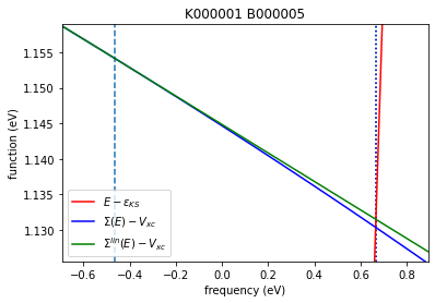
We see that eqpLin (green dotted line) and eqpSec (blue dotted line) correspond to the solution of the Quasiparticle equation with and without linearization of the frequency dependency, respectively.

[ ]: