This tutorial can be downloaded link.
1.0 Getting Started: GW calculation
In order to compute the GW electronic structure of the silane molecule you need to run pw.x, wstat.x and wfreq.x in sequence. Documentation for building and installing WEST is available at this link.
The GW workflow involves three sequental steps:
Step 1: Ground State
Step 2: Screening
Step 3: Quasiparticle corrections
Each step is explained below. At the end of step 3 you will be able to obtain the electronic structure of the silane molecule at the \(G_0W_0 @ PBE\) level of theory, where the GW is computed without empty states and with full frequency integration using the countour deformation technique. For more information about the implementation, we refer to Govoni et al., J. Chem. Theory Comput. 11, 2680 (2015).
Step 1: Ground State
The ground state electronic structure of silane molecule with Quantum ESPRESSO is obtained by running pw.x. Currently, WEST supports the version 6.8 of Quantum ESPRESSO. The pseudopotential files for Si and H in UPF format can be downloaded from: QE-PP database, or from SG15 database. Check out the pw.x input
description in order to generate an input file for Quantum ESPRESSO called pw.in.
Download these files in your current working directory:
[1]:
%%bash
wget -N -q http://www.west-code.org/doc/training/silane/pw.in
wget -N -q http://www.quantum-simulation.org/potentials/sg15_oncv/upf/H_ONCV_PBE-1.2.upf
wget -N -q http://www.quantum-simulation.org/potentials/sg15_oncv/upf/Si_ONCV_PBE-1.2.upf
Let’s inspect the pw.in file, input for pw.x.
[2]:
%%bash
cat pw.in
&control
calculation  = 'scf'
restart_mode = 'from_scratch'
pseudo_dir   = './'
outdir       = './'
prefix       = 'silane'
wf_collect   = .TRUE.
/
&system
ibrav           = 1
celldm(1)       = 20
nat             = 5
ntyp            = 2
ecutwfc         = 25.0
nbnd            = 10
assume_isolated ='mp'
/
&electrons
diago_full_acc = .TRUE.
/
ATOMIC_SPECIES
Si 28.0855  Si_ONCV_PBE-1.2.upf
H  1.00794   H_ONCV_PBE-1.2.upf
ATOMIC_POSITIONS bohr
Si      10.000000   10.000000  10.000000
H       11.614581   11.614581  11.614581
H        8.385418    8.385418  11.614581
H        8.385418   11.614581   8.385418
H       11.614581    8.385418   8.385418
K_POINTS {gamma}
Run pw.x on 2 cores.
[ ]:
%%bash
mpirun -n 2 pw.x < pw.in > pw.out
The output file pw.out contains information about the ground state calculation.
Step 2: Screening
The static dielectric screening is computed using the projective dielectric eigendecomposition (PDEP) technique. Check out the wstat.x input description and generate an input file for WEST called wstat.in.
Download this file in your current working directory:
[3]:
%%bash
wget -N -q http://www.west-code.org/doc/training/silane/wstat.in
Let’s inspect the wstat.in file, input for wstat.x.
[4]:
%%bash
cat wstat.in
input_west:
    qe_prefix: silane
    west_prefix: silane
    outdir: ./

wstat_control:
    wstat_calculation: S
    n_pdep_eigen: 50
Run wstat.x on 2 cores.
[ ]:
%%bash
mpirun -n 2 wstat.x -i wstat.in > wstat.out
The output file wstat.out contains information about the PDEP iterations, and the dielectric eigenvalues can be found in the file <west_prefix>.wstat.save/wstat.json.
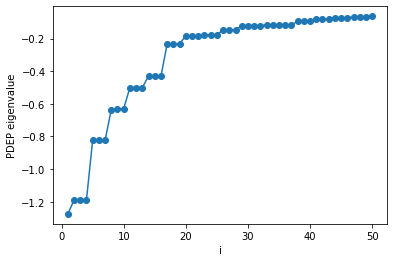
Below we show how to load, print, and plot the PDEP eigenvalues.
[5]:
import json
import numpy as np

# Load the output data
with open('silane.wstat.save/wstat.json') as json_file:
    data = json.load(json_file)

# Extract converged PDEP eigenvalues
ev = np.array(data["exec"]["davitr"][-1]["ev"],dtype="f8")
[6]:
# Print
print(ev)
[-1.27478021 -1.19127122 -1.19120182 -1.19117265 -0.82405876 -0.82403634
 -0.8239814  -0.63586048 -0.62939276 -0.62938952 -0.5005205  -0.50049623
 -0.50047244 -0.42993907 -0.42992203 -0.42991856 -0.23238121 -0.23237804
 -0.23237301 -0.18322991 -0.18321449 -0.18320583 -0.1783964  -0.17750084
 -0.17749955 -0.1459245  -0.14591779 -0.1459143  -0.12258015 -0.12012226
 -0.12011826 -0.12011616 -0.11634693 -0.11634526 -0.11528926 -0.11528499
 -0.11528457 -0.09408215 -0.09408058 -0.09408013 -0.07995372 -0.07995119
 -0.07995041 -0.07477358 -0.07310084 -0.07309955 -0.0657784  -0.06577326
 -0.06576894 -0.06313431]
[7]:
import matplotlib.pyplot as plt

# Create x-axis
iv = np.linspace(1,ev.size,ev.size,endpoint=True)

# Plot
plt.plot(iv,ev,'o-',label="XXX")
plt.xlabel("i")
plt.ylabel("PDEP eigenvalue")

plt.show()
Step 3: Quasiparticle corrections
The GW electronic structure is computed treating the frequency integration of the correlation part of the self energy with the Contour Deformation techinique and by computing the dielectric screening at multipole frequencies with Lanczos iterations. Check out the wfreq.x input description and generate an input file for WEST called wfreq.in.
Download this file in your current working directory:
[8]:
%%bash
wget -N -q http://www.west-code.org/doc/training/silane/wfreq.in
Let’s inspect the wfreq.in file, input for wfreq.x.
[9]:
%%bash
cat wfreq.in
input_west:
    qe_prefix: silane
    west_prefix: silane
    outdir: ./

wstat_control:
    wstat_calculation: S
    n_pdep_eigen: 50

wfreq_control:
    wfreq_calculation: XWGQ
    n_pdep_eigen_to_use: 50
    qp_bandrange: [1,5]
    n_refreq: 300
    ecut_refreq: 2.0
Run wfreq.x on 2 cores.
[ ]:
%%bash
mpirun -n 2 wfreq.x -i wfreq.in > wfreq.out
The output file wfreq.out contains information about the calculation of the GW self-energy, and the corrected electronic structure can be found in the file <west_prefix>.wfreq.save/wfreq.json.
Below we show how to load, print, and plot the quasiparticle corrections.
[10]:
import json
import numpy as np

# Load the output data
with open('silane.wfreq.save/wfreq.json') as json_file:
    data = json.load(json_file)

# Extract converged quasiparticle (QP) corrections
k=1
kindex = f"K{k:06d}"

bandmap = data["output"]["Q"]["bandmap"]
eqp = data["output"]["Q"][kindex]
[11]:
# Print QP corrections
print (f"{'k':^10} | {'band':^10} | {'eks [eV]':^15} | {'eqpLin [eV]':^15} | {'eqpSec [eV]':^15}")
print(77*"-")
for i, b in enumerate(bandmap) :
    print(f"{k:^10} | {b:^10} | {eqp['eks'][i]:^15.3f} | {eqp['eqpLin'][i]:^15.3f} | {eqp['eqpSec'][i]:^15.3f}")
    k      |    band    |    eks [eV]     |   eqpLin [eV]   |   eqpSec [eV]
-----------------------------------------------------------------------------
    1      |     4      |     -8.230      |     -12.150     |     -12.044
    1      |     5      |     -0.466      |      0.666      |      0.665
Explanation of keys:
eks: Kohn-Sham energy (obtained in Step 1)eqpLin: Quasiparticle energy (\(G_0W_0 @ PBE\)), obtained by approximating the self-energy to first order in the frequencyeqpSec: Quasiparticle energy (\(G_0W_0 @ PBE\))
[ ]: