This tutorial can be downloaded link.

Intro Tutorial 2: Analyzing the Frequency Dependency in GW Calculations

We analyze the frequency dependency of the GW self-energy, by exploring two ways of solving the quasiparticle (QP) equation:

• without linearization

\begin{equation} E - \varepsilon_{\mathrm{KS}} = \langle \Sigma(E) - V_{\mathrm{xc}} \rangle \end{equation}

• with linearization (first-order expansion of self-energy in the frequency domain)

\begin{equation} E - \varepsilon_{\mathrm{KS}} = \langle \Sigma(\varepsilon_{\mathrm{KS}}) - V_{\mathrm{xc}} \rangle + (E - \varepsilon_{\mathrm{KS}}) \langle \frac{\partial \Sigma}{\partial E}(\varepsilon_{\mathrm{KS}}) \rangle \end{equation}

where \(\varepsilon_{\mathrm{KS}}\) is the Kohn-Sham energy, \(\Sigma\) is the real part of the self energy, \(V_{\mathrm{xc}}\) is the exchange-correlation potential, and the solution \(E\) is the QP energy obtained at the \(G_0W_0\) level of theory.

After completing step 1 and step 2 of Tutorial 1, we download the following file:

%%bash
wget -N -q https://west-code.org/doc/training/silane/wfreq_spec.in

Let’s inspect the wfreq_spec.in file, input for wfreq.x.

%%bash
cat wfreq_spec.in

input_west:
    qe_prefix: silane
    west_prefix: silane
    outdir: ./

wstat_control:
    wstat_calculation: S
    n_pdep_eigen: 50

wfreq_control:
    wfreq_calculation: XWGQP
    n_pdep_eigen_to_use: 50
    qp_bandrange: [4,5]
    n_refreq: 2000
    ecut_refreq: 2.0
    ecut_spectralf: [-1.5,0.5]
    n_spectralf: 2000

The keyword ecut_spectralf: [-1.5,0.5] activates the computation of the self energy in the frequency range of [-1.5,0.5] Ry.

We run wfreq.x on 2 cores.

%%bash
mpirun -n 2 wfreq.x -i wfreq_spec.in > wfreq_spec.out

The output file wfreq.out contains information about the GW calculation, and the corrected electronic structure can be found in the file <west_prefix>.wfreq.save/wfreq.json.

If the reader does NOT have the computational resources to run the calculation, the WEST output file needed for the next step can be directly downloaded as:

%%bash
mkdir -p silane.wfreq.save
wget -N -q https://west-code.org/doc/training/silane/wfreq_spec.json -O silane.wfreq.save/wfreq.json

Below we show how to load and plot the frequency-dependent QP corrections.

import json
import numpy as np

# Load the output data
with open('silane.wfreq.save/wfreq.json') as json_file :
    data = json.load(json_file)

# Extract converged quasiparticle (QP) corrections
k = 1
kindex = f'K{k:06d}'

qp_bands = data['input']['wfreq_control']['qp_bands'][0]
eqp = data['output']['Q'][kindex]

freqlist = np.array(data['output']['P']['freqlist'], dtype='f8')
spf = data['output']['P'][kindex]

# Plot
import matplotlib.pyplot as plt

for i, b in enumerate(qp_bands) :

    eks, eqpLin, eqpSec = eqp['eks'][i], eqp['eqpLin'][i], eqp['eqpSec'][i]

    # Print QP corrections
    print (f"{'k':^10} | {'band':^10} | {'eks [eV]':^15} | {'eqpLin [eV]':^15} | {'eqpSec [eV]':^15}")
    print(77*'-')
    print(f'{k:^10} | {b:^10} | {eks:^15.3f} | {eqpLin:^15.3f} | {eqpSec:^15.3f}')

    sigmax, vxcl, vxcnl = eqp['sigmax'][i], eqp['vxcl'][i], eqp['vxcnl'][i]
    sigmac_eks = eqp['sigmac_eks']['re'][i]
    sigmac_eqpLin = eqp['sigmac_eqpLin']['re'][i]
    sigmac_eqpSec = eqp['sigmac_eqpSec']['re'][i]
    z = eqp['z'][i]

    bindex = f'B{b:06d}'
    sigmac = np.array(spf[bindex]['sigmac']['re'], dtype='f8')

    # Left-hand side of QP equation
    plt.plot(freqlist,freqlist-eks,'r-',label=r'$E-\varepsilon_{KS}$')

    # Right-hand side of QP equation without linearization
    plt.plot(freqlist,sigmac+sigmax-vxcl-vxcnl,'b-',label=r'$\Sigma(E)-V_{xc}$')

    # Right-hand side of QP equation with linearization
    plt.plot(freqlist,sigmac_eks+sigmax-vxcl-vxcnl+(1-1/z)*(freqlist-eks),'g-',label=r'$\Sigma^{lin}(E)-V_{xc}$')

    plt.legend()
    plt.title(kindex+" "+bindex)
    plt.xlabel('frequency (eV)')
    plt.ylabel('function (eV)')
    xmin, xmax = min(eks, eqpLin, eqpSec), max(eks, eqpLin, eqpSec)
    ymin, ymax = min(sigmac_eks, sigmac_eqpLin, sigmac_eqpSec), max(sigmac_eks, sigmac_eqpLin, sigmac_eqpSec)
    ymin += sigmax - vxcl -vxcnl
    ymax += sigmax - vxcl -vxcnl
    plt.vlines(x=eks,ymin=ymin-0.2*(ymax-ymin),ymax=ymax+0.2*(ymax-ymin),ls="--")
    plt.vlines(x=eqpLin,ymin=ymin-0.2*(ymax-ymin),ymax=ymax+0.2*(ymax-ymin),ls=":",color="g")
    plt.vlines(x=eqpSec,ymin=ymin-0.2*(ymax-ymin),ymax=ymax+0.2*(ymax-ymin),ls=":",color="b")
    plt.xlim([xmin-0.2*(xmax-xmin),xmax+0.2*(xmax-xmin)])
    plt.ylim([ymin-0.2*(ymax-ymin),ymax+0.2*(ymax-ymin)])
    plt.show()

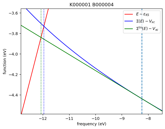
    k      |    band    |    eks [eV]     |   eqpLin [eV]   |   eqpSec [eV]
-----------------------------------------------------------------------------
    1      |     4      |     -8.232      |     -12.071     |     -11.962

    k      |    band    |    eks [eV]     |   eqpLin [eV]   |   eqpSec [eV]
-----------------------------------------------------------------------------
    1      |     5      |     -0.466      |      0.589      |      0.587

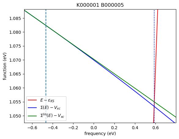
In the above plots, the red, blue, and green solid lines represent \(E - \varepsilon_{\mathrm{KS}}\), \(\Sigma (E) - V_{\mathrm{XC}}\), and \(\Sigma^{\mathrm{lin}} (E) - V_{\mathrm{XC}}\), respectively. The intersection of the red and blue solid lines, marked by the blue dotted line, corresponds to the solution (eqpSec) of the QP equation without linearization of the frequency dependency. Likewise, the intersection of the red and green solid lines, marked by the green dotted line, corresponds to the solution (eqpLin) of the QP equation with linearization.