This tutorial can be downloaded link.

Intro tutorial 6: Identification of localized states

In this tutorial, we show how to identify Kohn-Sham states that are localized in real space. We will identify defect orbitals of the \(\mathrm{NV^-}\) center in diamond based on the localization factor, defined as

\[L_n = \int_{V \in \Omega} d^3\mathbf{r} \left| \psi^{\text{KS}}_n(\mathbf{r}) \right|^2\]

It describes the localization of the n-th KS wavefunction in a given volume \(V\) within the supercell volume \(\Omega\). The volume \(V\) can be a box or a sphere.

More details can be found in N. Sheng, C. Vorwerk, M. Govoni, and G. Galli, J. Chem. Theory Comput. 18, 6, 3512 (2022).

Step 1: Mean-field starting point

As a first step, we perform the mean-field electronic structure calculation within density-functional theory (DFT) using the Quantum ESPRESSO code.

Download the following files in your working directory:

%%bash
wget -N -q http://www.west-code.org/doc/training/nv_diamond_63/pw.in
wget -N -q http://www.quantum-simulation.org/potentials/sg15_oncv/upf/C_ONCV_PBE-1.0.upf
wget -N -q http://www.quantum-simulation.org/potentials/sg15_oncv/upf/N_ONCV_PBE-1.0.upf

We can now inspect the pw.in file, the input for the pw.x code:

%%bash
cat pw.in

&CONTROL
calculation = 'scf'
wf_collect = .true.
pseudo_dir = './'
/
&SYSTEM
input_dft = 'PBE'
ibrav = 0
ecutwfc = 50
nosym = .true.
tot_charge = -1
nspin = 1
nbnd = 176
occupations = 'from_input'
nat = 63
ntyp = 2
/
&ELECTRONS
conv_thr = 1D-08
/
K_POINTS gamma
CELL_PARAMETERS angstrom
7.136012  0.000000  0.000000
0.000000  7.136012  0.000000
0.000000  0.000000  7.136012
ATOMIC_SPECIES
C  12.01099968  C_ONCV_PBE-1.0.upf
N  14.00699997  N_ONCV_PBE-1.0.upf
ATOMIC_POSITIONS crystal
C    0.99996000  0.99996000  0.99996000
C    0.12495000  0.12495000  0.12495000
C    0.99905000  0.25039000  0.25039000
C    0.12350000  0.37499000  0.37499000
C    0.25039000  0.99905000  0.25039000
C    0.37499000  0.12350000  0.37499000
C    0.25039000  0.25039000  0.99905000
C    0.37499000  0.37499000  0.12350000
C    0.00146000  0.00146000  0.50100000
C    0.12510000  0.12510000  0.62503000
C    0.00102000  0.24944000  0.74960000
C    0.12614000  0.37542000  0.87402000
C    0.24944000  0.00102000  0.74960000
C    0.37542000  0.12614000  0.87402000
C    0.24839000  0.24839000  0.49966000
C    0.37509000  0.37509000  0.61906000
C    0.00146000  0.50100000  0.00146000
C    0.12510000  0.62503000  0.12510000
C    0.00102000  0.74960000  0.24944000
C    0.12614000  0.87402000  0.37542000
C    0.24839000  0.49966000  0.24839000
C    0.37509000  0.61906000  0.37509000
C    0.24944000  0.74960000  0.00102000
C    0.37542000  0.87402000  0.12614000
C    0.99883000  0.50076000  0.50076000
C    0.12502000  0.62512000  0.62512000
C    0.99961000  0.74983000  0.74983000
C    0.12491000  0.87493000  0.87493000
C    0.25216000  0.50142000  0.74767000
C    0.37740000  0.62659000  0.87314000
C    0.25216000  0.74767000  0.50142000
C    0.37740000  0.87314000  0.62659000
C    0.50100000  0.00146000  0.00146000
C    0.62503000  0.12510000  0.12510000
C    0.49966000  0.24839000  0.24839000
C    0.61906000  0.37509000  0.37509000
C    0.74960000  0.00102000  0.24944000
C    0.87402000  0.12614000  0.37542000
C    0.74960000  0.24944000  0.00102000
C    0.87402000  0.37542000  0.12614000
C    0.50076000  0.99883000  0.50076000
C    0.62512000  0.12502000  0.62512000
C    0.50142000  0.25216000  0.74767000
C    0.62659000  0.37740000  0.87314000
C    0.74983000  0.99961000  0.74983000
C    0.87493000  0.12491000  0.87493000
C    0.74767000  0.25216000  0.50142000
C    0.87314000  0.37740000  0.62659000
C    0.50076000  0.50076000  0.99883000
C    0.62512000  0.62512000  0.12502000
C    0.50142000  0.74767000  0.25216000
C    0.62659000  0.87314000  0.37740000
C    0.74767000  0.50142000  0.25216000
C    0.87314000  0.62659000  0.37740000
C    0.74983000  0.74983000  0.99961000
C    0.87493000  0.87493000  0.12491000
N    0.48731000  0.48731000  0.48731000
C    0.49191000  0.76093000  0.76093000
C    0.62368000  0.87476000  0.87476000
C    0.76093000  0.49191000  0.76093000
C    0.87476000  0.62368000  0.87476000
C    0.76093000  0.76093000  0.49191000
C    0.87476000  0.87476000  0.62368000
OCCUPATIONS
2.00  2.00  2.00  2.00  2.00  2.00  2.00  2.00  2.00  2.00
2.00  2.00  2.00  2.00  2.00  2.00  2.00  2.00  2.00  2.00
2.00  2.00  2.00  2.00  2.00  2.00  2.00  2.00  2.00  2.00
2.00  2.00  2.00  2.00  2.00  2.00  2.00  2.00  2.00  2.00
2.00  2.00  2.00  2.00  2.00  2.00  2.00  2.00  2.00  2.00
2.00  2.00  2.00  2.00  2.00  2.00  2.00  2.00  2.00  2.00
2.00  2.00  2.00  2.00  2.00  2.00  2.00  2.00  2.00  2.00
2.00  2.00  2.00  2.00  2.00  2.00  2.00  2.00  2.00  2.00
2.00  2.00  2.00  2.00  2.00  2.00  2.00  2.00  2.00  2.00
2.00  2.00  2.00  2.00  2.00  2.00  2.00  2.00  2.00  2.00
2.00  2.00  2.00  2.00  2.00  2.00  2.00  2.00  2.00  2.00
2.00  2.00  2.00  2.00  2.00  2.00  2.00  2.00  2.00  2.00
2.00  2.00  2.00  2.00  2.00  2.00  1.00  1.00  0.00  0.00
0.00  0.00  0.00  0.00  0.00  0.00  0.00  0.00  0.00  0.00
0.00  0.00  0.00  0.00  0.00  0.00  0.00  0.00  0.00  0.00
0.00  0.00  0.00  0.00  0.00  0.00  0.00  0.00  0.00  0.00
0.00  0.00  0.00  0.00  0.00  0.00  0.00  0.00  0.00  0.00
0.00  0.00  0.00  0.00  0.00  0.00

We can now run pw.x on 2 cores.

%%bash
mpirun -n 2 pw.x -i pw.in > pw.out

We have carried out a spin unpolarized calculation (i.e., nspin = 1) because we want to use \(L_n\) to define an active space for quantum defect embedding theory (QDET, see Tutorial 5). The latter uses a spin-unpolarized mean-field starting point to reduce spin contamination in the generation of the parameters for the effective Hamiltonian.

Step 2.1: Calculation of the localization factor using a box

Localization factors are calculated with the westpp.x executable within WEST. You can download the input file with the following command:

%%bash
wget -N -q http://www.west-code.org/doc/training/nv_diamond_63/westpp.in

Let us inspect the input file.

%%bash
cat westpp.in

wstat_control:
  wstat_calculation: S
  n_pdep_eigen: 512

westpp_control:
  westpp_calculation: L
  westpp_range: [1, 176]
  westpp_box: [6.19, 10.19, 6.28, 10.28, 6.28, 10.28]

The keyword westpp_calculation: L triggers the calculation of the localization factor. With westpp_range, we can select for which Kohn-Sham states we compute the localization factor. In this tutorial, we use all 176 states. Finally, westpp_box specifies the parameter of a box in atomic units to use for the integration. In this case, we have chosen a cubic box around the carbon vacancy at \(\left( 8.18, 8.28, 8.28 \right)\) Bohr with an edge of 4 Bohr. The box has a volume of 64 Bohr\(^3\), which is smaller than the supercell volume of 2452.24 Bohr\(^3\).

Run westpp.x on 2 cores.

%%bash
mpirun -n 2 westpp.x -i westpp.in > westpp.out

westpp.x creates a file named west.westpp.save/localization.json. If the reader does NOT have the computational resources to run the calculation, the WEST output file needed for the next step can be directly downloaded as:

%%bash
mkdir -p west.westpp.save
wget -N -q http://www.west-code.org/doc/training/nv_diamond_63/localization.json -O west.westpp.save/localization.json

We can now visualize the results:

import json
import numpy as np
import matplotlib.pyplot as plt

with open('west.westpp.save/localization.json','r') as f:
    data = json.load(f)

y = np.array(data['localization'],dtype='f8')
x = np.array([i+1 for i in range(y.shape[0])])

plt.plot(x,y,'o')
plt.axhline(y=0.08,linestyle='--',color='red')


plt.xlabel(r'$\mathrm{KS \; Index}$')
plt.ylabel(r'$\mathrm{Localization \; Factor}$')

plt.show()

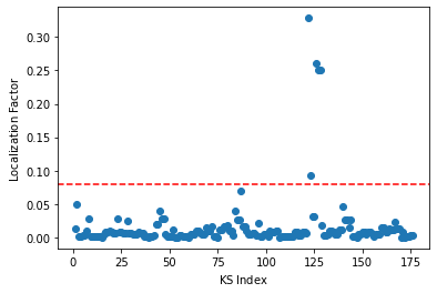
We see that a number of Kohn-Sham orbitals have a localization factor \(>0.08\).

print(x[y>=0.08])

[122 123 126 127 128]

The highest localization factor (>0.08) is found for Kohn-Sham orbitals with indices 122, 123, 126, 127, and 128.

Step 2.2: Calculation of the localization factor using a sphere

Let us modify the input file westpp.in to compute localization factors within a sphere.

import yaml

with open('westpp.in') as file:
    input_data = yaml.load(file, Loader=yaml.FullLoader)

input_data['westpp_control']['westpp_calculation'] = 'L'
input_data['westpp_control']['westpp_format'] = 'S'
input_data['westpp_control']['westpp_r0'] = [8.18, 8.28, 8.28]
input_data['westpp_control']['westpp_rmax'] = 2.4814

with open('westpp.in', 'w') as file:
    yaml.dump(input_data, file, sort_keys=False)

Let us inspect the input file.

%%bash
cat westpp.in

wstat_control:
  wstat_calculation: S
  n_pdep_eigen: 512
westpp_control:
  westpp_calculation: L
  westpp_range:
  - 1
  - 176
  westpp_box:
  - 6.19
  - 10.19
  - 6.28
  - 10.28
  - 6.28
  - 10.28
  westpp_format: S
  westpp_r0:
  - 8.18
  - 8.28
  - 8.28
  westpp_rmax: 2.4814

The keyword westpp_format: S instructs the code to compute the localization factor within a sphere, which is centered around \(\left( 8.18, 8.28, 8.28 \right)\) Bohr as specified by westpp_r0 and has a radius of 2.4814 Bohr as specified by westpp_rmax. The sphere has a volume of ~64 Bohr\(^3\), which is roughly the same as the volume of the box used in the previous section.

Run westpp.x on 2 cores.

%%bash
mpirun -n 2 westpp.x -i westpp.in > westpp.out

westpp.x creates a file named west.westpp.save/localization.json. If the reader does NOT have the computational resources to run the calculation, the WEST output file needed for the next step can be directly downloaded as:

%%bash
mkdir -p west.westpp.save
wget -N -q http://www.west-code.org/doc/training/nv_diamond_63/localization2.json -O west.westpp.save/localization.json

We can now visualize the results:

import json
import numpy as np
import matplotlib.pyplot as plt

with open('west.westpp.save/localization.json','r') as f:
    data = json.load(f)

y = np.array(data['localization'],dtype='f8')
x = np.array([i+1 for i in range(y.shape[0])])

plt.plot(x,y,'o')
plt.axhline(y=0.08,linestyle='--',color='red')

plt.xlabel(r'$\mathrm{KS \; Index}$')
plt.ylabel(r'$\mathrm{Localization \; Factor}$')

plt.show()

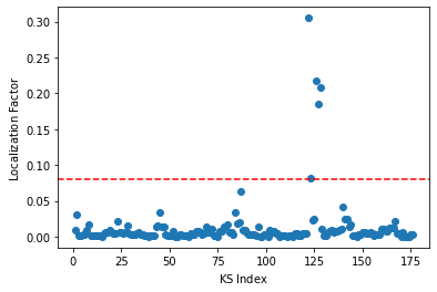
We see that a number of Kohn-Sham orbitals have a localization factor \(>0.08\).

print(x[y>=0.08])

[122 123 126 127 128]

The highest localization factor (>0.08) is found for Kohn-Sham orbitals with indices 122, 123, 126, 127, and 128, which are the same orbitals as identified by computing localization factors in a box.